Fit Tensor to RDC Data

This example shows how to fit a \({\Delta\chi}\)-tensor or equivalently, and alignment tensor to experimental RDC data. These data are taken from a Tb3+ tagged ubiquitin mutant:

Benjamin J. G. Pearce, Shereen Jabar, Choy-Theng Loh, Monika Szabo, Bim Graham, Gottfried Otting (2017) Structure restraints from heteronuclear pseudocontact shifts generated by lanthanide tags at two different sites J. Biomol. NMR 68:19-32

Downloads

• Download the data files 2kox.pdb, ubiquitin_a28c_c1_Tb_HN.rdc and ubiquitin_s57c_c1_Tb_HN.rdc from here:

• Download the script rdc_fit.py

Script + Explanation

Firstly, the necessary modules are imported from paramagpy. And the two RDC datasets are loaded. Because this PDB contains over 600 models, loading may take a few seconds

from paramagpy import protein, fit, dataparse, metal

# Load the PDB file
prot = protein.load_pdb('../data_files/2kox.pdb')

# Load the RDC data
rawData1 = dataparse.read_rdc('../data_files/ubiquitin_a28c_c1_Tb_HN.rdc')
rawData2 = dataparse.read_rdc('../data_files/ubiquitin_s57c_c1_Tb_HN.rdc')

# Associate RDC data with atoms of the PDB
parsedData1 = prot.parse(rawData1)
parsedData2 = prot.parse(rawData2)

Two starting metals are initialised. It is important here to set the magnetic field strength and temperature.

# Define an initial tensor
mStart1 = metal.Metal(B0=18.8, temperature=308.0)
mStart2 = metal.Metal(B0=18.8, temperature=308.0)

The alignment tensor is solved using the function paramagpy.fit.svd_fit_metal_from_rdc() which return a tuple of (metal, calculated), where metal is the fitted metal, calculated is the calculated RDC values. The tensors are then saved. Note that we set the argument ensembleAverage to True. This is important because the PDB structure represents and MD simulation. If set to False, a much smaller tensor would be fit.

# Calculate the tensor using SVD
[sol1], [data1] = fit.svd_fit_metal_from_rdc([mStart1], [parsedData1], ensembleAverage=True)
[sol2], [data2] = fit.svd_fit_metal_from_rdc([mStart2], [parsedData2], ensembleAverage=True)

# Save the fitted tensor to file
sol1.save('ubiquitin_a28c_c1_Tb_tensor.txt')
sol2.save('ubiquitin_s57c_c1_Tb_tensor.txt')

Output: [ubiquitin_a28c_c1_Tb_tensor.txt]

ax    | 1E-32 m^3 :    -4.776
rh    | 1E-32 m^3 :    -1.397
x     |   1E-10 m :     0.000
y     |   1E-10 m :     0.000
z     |   1E-10 m :     0.000
a     |       deg :    16.022
b     |       deg :    52.299
g     |       deg :    83.616
mueff |        Bm :     0.000
shift |       ppm :     0.000
B0    |         T :    18.800
temp  |         K :   308.000
t1e   |        ps :     0.000
taur  |        ns :     0.000

Output: [ubiquitin_s57c_c1_Tb_tensor.txt]

ax    | 1E-32 m^3 :    -5.930
rh    | 1E-32 m^3 :    -1.899
x     |   1E-10 m :     0.000
y     |   1E-10 m :     0.000
z     |   1E-10 m :     0.000
a     |       deg :     9.976
b     |       deg :    99.463
g     |       deg :    37.410
mueff |        Bm :     0.000
shift |       ppm :     0.000
B0    |         T :    18.800
temp  |         K :   308.000
t1e   |        ps :     0.000
taur  |        ns :     0.000

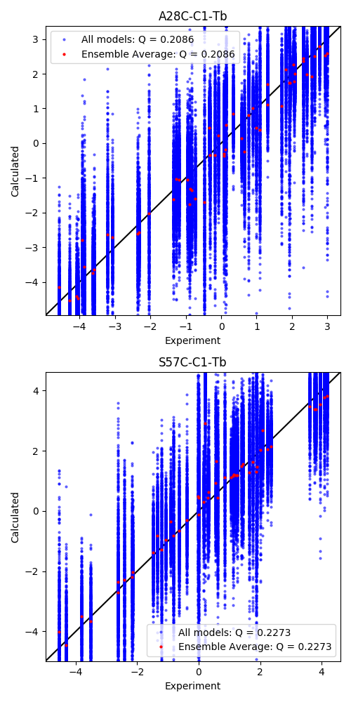
The experimental/calculated correlations are then plotted. The tensor is by default fitted to the ensemble averaged calculated values. Backcalculation of all models is shown here, as well as the ensemble average.

#### Plot the correlation ####
from matplotlib import pyplot as plt
fig = plt.figure(figsize=(5,10))
ax1 = fig.add_subplot(211)
ax2 = fig.add_subplot(212)
ax1.set_title('A28C-C1-Tb')
ax2.set_title('S57C-C1-Tb')

for sol, ax, data in zip([sol1,sol2], [ax1,ax2], [data1,data2]):

	# Calculate ensemble averages
	dataEAv = fit.ensemble_average(data)

	# Calculate the Q-factor
	qfac = fit.qfactor(data, ensembleAverage=True)

	# Plot all models
	ax.plot(data['exp'], data['cal'], marker='o', lw=0, ms=2, c='b', 
		alpha=0.5, label="All models: Q = {:5.4f}".format(qfac))

	# Plot the ensemble average
	ax.plot(dataEAv['exp'], dataEAv['cal'], marker='o', lw=0, ms=2, c='r', 
		label="Ensemble Average: Q = {:5.4f}".format(qfac))

	# Plot a diagonal
	l, h = ax.get_xlim()
	ax.plot([l,h],[l,h],'-k',zorder=0)
	ax.set_xlim(l,h)
	ax.set_ylim(l,h)

	# Make axis labels and save figure
	ax.set_xlabel("Experiment")
	ax.set_ylabel("Calculated")
	ax.legend()

fig.tight_layout()
fig.savefig("rdc_fit.png")

Output: [rdc_fit.png]