Fit Tensor to PCS Data
This example shows how to fit a \({\Delta\chi}\)-tensor to experimental PCS data for the protein calbindin D9k. These data contain amide 1H and 15N chemical shifts between diamagnetic and paramagnetic states with the lanthanide Er3+ bound.
Downloads
Download the data files
4icbH_mut.pdbandcalbindin_Er_HN_PCS.npcfrom here:Download the script
pcs_fit.py
Script + Explanation
Firstly, the necessary modules are imported from paramagpy.
from paramagpy import protein, fit, dataparse, metal
The protein is then loaded from a PDB file using paramagpy.protein.load_pdb() into the variable prot. This returns a CustomStructure object which is closely based on the Structure object from BioPython and contains the atomic coordinates. The object, and how to access atomic coordinates is discussed at this link.
# Load the PDB file
prot = protein.load_pdb('../data_files/4icbH_mut.pdb')
The PCS data is then loaded from a .npc file using the function paramagpy.dataparse.read_pcs() into the variable rawData. This is a dictionary of (PCS, Error) tuples which may be accessed by rawData[(seq, atom)] where seq is an integer specifying the sequence and atom is the atom name e.g (3,'HA'). Note that these should match the corresponding sequence and atom in the PDB file.
# Load the PCS data
rawData = dataparse.read_pcs('../data_files/calbindin_Er_HN_PCS.npc')
To associate the experimental PCS value with atoms of the PDB structure, the method paramagpy.protein.CustomStructure.parse() is called on rawData. The returned array parsedData has a row for each atom with columns [mdl,atm,exp,cal,err,idx], where mdl is the model number from the PDB file, atm is an atom object from the BioPython PDB structure, exp and cal are the experimental and calculated values, err is the experimental uncertainty and idx is the atom index, used to define ensemble averaging behaviour.
# Associate PCS data with atoms of the PDB
parsedData = prot.parse(rawData)
An initial \({\Delta\chi}\)-tensor is defined by initialising a paramagpy.metal.Metal object. The initial position is known to be near the binding site, which is set to the CA atom of residue 56. Note that the position attribute is always in Angstrom units.
# Define an initial tensor
mStart = metal.Metal()

# Set the starting position to an atom close to the metal
mStart.position = prot[0]['A'][56]['CA'].position
A quick gridsearch is conducted in a sphere of 10 Angstrom with 10 points per radius using the function paramagpy.fit.svd_gridsearch_fit_metal_from_pcs(). This requires two lists containing the starting metals mStart and parsed experimental dataArray parsedData. This function returns lists containing a new fitted metal object, the calculated PCS values from the fitted model.
# Calculate an initial tensor from an SVD gridsearch
[mGuess], [data] = fit.svd_gridsearch_fit_metal_from_pcs(
	[mStart],[parsedData], radius=10, points=10)
This is then refined using a non-linear regression gradient descent with the function paramagpy.fit.nlr_fit_metal_from_pcs().
# Refine the tensor using non-linear regression
[mFit], [data] = fit.nlr_fit_metal_from_pcs([mGuess], [parsedData])
The Q-factor is then calculated using the function :py:func`paramagpy.fit.qfactor`.
# Calculate the Q-factor
qfac = fit.qfactor(data)
The fitted tensor parameters are saved by calling the method paramagpy.metal.Metal.save(). Alterntaively they may be displayed using print(mFit.info())
# Save the fitted tensor to file
mFit.save('calbindin_Er_HN_PCS_tensor.txt')
Output: [calbindin_Er_HN_PCS_tensor.txt]
ax    | 1E-32 m^3 :    -8.688
rh    | 1E-32 m^3 :    -4.192
x     |   1E-10 m :    25.517
y     |   1E-10 m :     8.652
z     |   1E-10 m :     6.358
a     |       deg :   116.011
b     |       deg :   138.058
g     |       deg :    43.492
mueff |        Bm :     0.000
shift |       ppm :     0.000
B0    |         T :    18.790
temp  |         K :   298.150
t1e   |        ps :     0.000
taur  |        ns :     0.000
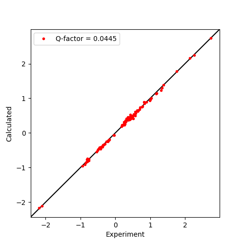
These experimental/calculated PCS values are then plotted in a correlation plot to assess the fit. This is achieved using standard functions of the plotting module matplotlib.
#### Plot the correlation ####
from matplotlib import pyplot as plt
fig, ax = plt.subplots(figsize=(5,5))

# Plot the data
ax.plot(data['exp'], data['cal'], marker='o', lw=0, ms=3, c='r',
	label="Q-factor = {:5.4f}".format(qfac))

# Plot a diagonal
l, h = ax.get_xlim()
ax.plot([l,h],[l,h],'-k',zorder=0)
ax.set_xlim(l,h)
ax.set_ylim(l,h)

# Make axis labels and save figure
ax.set_xlabel("Experiment")
ax.set_ylabel("Calculated")
ax.legend()
fig.savefig("pcs_fit.png")
Output: [pcs_fit.png]