Fit Tensor to PRE Data

This example demonstrates fitting of the rotational correlation time \({\tau_r}\) to 1H PRE data of calbindin D9k. You can fit any parameters of the \({\chi}\)-tensor you desire, such as position or magnitude as well.

Downloads

• Download the data files 4icbH_mut.pdb, calbindin_Er_H_R2_600.npc and calbindin_Tb_H_R2_800.npc from here:

• Download the script pre_fit_proton.py

Script + Explanation

Firstly, the necessary modules are imported from paramagpy.

from paramagpy import protein, fit, dataparse, metal

The protein is then loaded from a PDB file.

# Load the PDB file
prot = protein.load_pdb('../data_files/4icbH_mut.pdb')

The PRE data is loaded. Note that the Er data was recorded at 600 MHz and the Tb data was recorded at 800 MHz.

rawData_er = dataparse.read_pre('../data_files/calbindin_Er_H_R2_600.pre')
rawData_tb = dataparse.read_pre('../data_files/calbindin_Tb_H_R2_800.pre')

The \({\Delta\chi}\)-tensors that were fitted from PCS data are loaded from file and the relevant \({B_0}\) magnetic field strengths are set.

mStart_er = metal.load_tensor('../data_files/calbindin_Er_HN_PCS_tensor.txt')
mStart_tb = metal.load_tensor('../data_files/calbindin_Tb_HN_PCS_tensor.txt')
mStart_er.B0 = 14.1
mStart_tb.B0 = 18.8

Fitting of the rotational correlation time is done with the function paramagpy.fit.nlr_fit_metal_from_pre(). To fit position or \({\chi}\)-tensor magnitude, you can change the params argument.

(m_er,), (cal_er,) = fit.nlr_fit_metal_from_pre(
	[mStart_er], [data_er], params=['taur'], rtypes=['r2'])
(m_tb,), (cal_tb,) = fit.nlr_fit_metal_from_pre(
	[mStart_tb], [data_tb], params=['taur'], rtypes=['r2'])

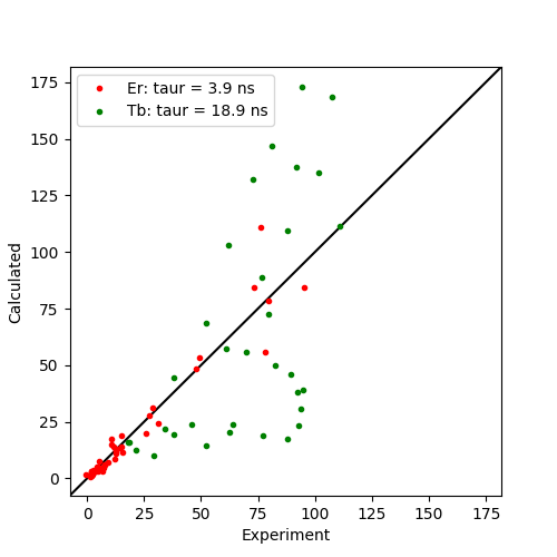
The fitted tensors are saved to file. Note that the Er dataset gives a reasonable \({\tau_r}\) of around 4 ns which is close to the literature value of 4.25 ns. However, the Tb dataset gives an unreasonably large value of 18 ns. This is due to magnetisation attenuation due to 1H-1H RDCs present during the relaxation evolution time as discussed in literature giving rise to artificially large measured PREs for lanthanides with highly anisotropic \({\Delta\chi}\)-tensors. This is also reflected in the correlation plot below.

m_er.save('calbindin_Er_H_R2_600_tensor.txt')
m_tb.save('calbindin_Tb_H_R2_800_tensor.txt')

Output: [calbindin_Er_H_R2_600_tensor.txt]

ax    | 1E-32 m^3 :    -8.152
rh    | 1E-32 m^3 :    -4.911
x     |   1E-10 m :    25.786
y     |   1E-10 m :     9.515
z     |   1E-10 m :     6.558
a     |       deg :   125.841
b     |       deg :   142.287
g     |       deg :    41.758
mueff |        Bm :     9.581
shift |       ppm :     0.000
B0    |         T :    14.100
temp  |         K :   298.150
t1e   |        ps :     0.189
taur  |        ns :     3.923

Output: [calbindin_Tb_H_R2_800_tensor.txt]

ax    | 1E-32 m^3 :    30.375
rh    | 1E-32 m^3 :    12.339
x     |   1E-10 m :    25.786
y     |   1E-10 m :     9.515
z     |   1E-10 m :     6.558
a     |       deg :   150.957
b     |       deg :   152.671
g     |       deg :    70.311
mueff |        Bm :     9.721
shift |       ppm :     0.000
B0    |         T :    18.800
temp  |         K :   298.150
t1e   |        ps :     0.251
taur  |        ns :    18.917

And the results are plotted.

from matplotlib import pyplot as plt
fig, ax = plt.subplots(figsize=(5,5))

# Plot the data
ax.plot(cal_er['exp'], cal_er['cal'], marker='o', lw=0, ms=3, c='r',
	label="Er: taur = {:3.1f} ns".format(1E9*m_er.taur))
ax.plot(cal_tb['exp'], cal_tb['cal'], marker='o', lw=0, ms=3, c='g',
	label="Tb: taur = {:3.1f} ns".format(1E9*m_tb.taur))

# Plot a diagonal
l, h = ax.get_ylim()
ax.plot([l,h],[l,h],'-k',zorder=0)
ax.set_xlim(l,h)
ax.set_ylim(l,h)

# Make axis labels and save figure
ax.set_xlabel("Experiment")
ax.set_ylabel("Calculated")
ax.legend()
fig.savefig("pre_fit_proton.png")