Calculate Cross-correlated Relaxation
This example shows how to calculate dipole-dipole/Curie-spin cross-correlated relaxation as measured for data in the literature by Pintacuda et. al.
Downloads
Download the data files
1bzrH.pdb,myoglobin_cn.ccrandmyoglobin_f.ccrfrom here:Download the script
ccr_calculate.py
Script + Explanation
First the relevant modules are loaded, and the iron atom (paramagnetic centre) is identified as the variable ironAtom.
from paramagpy import protein, fit, dataparse, metal
import numpy as np

# Load the PDB file and get iron centre
prot = protein.load_pdb('../data_files/1bzrH.pdb')
ironAtom = prot[0]['A'][("H_HEM",154," ")]['FE']
Two paramagnetic centres are defined for the high and low spin iron atom. The positions are set to that of the iron centre along with other relevant parameters. The measured isotropic \({\chi}\)-tensor magnitudes are also set.
met_cn = metal.Metal(position=ironAtom.position,
					 B0=18.79,
					 temperature=303.0,
					 taur=5.7E-9)
met_f = met_cn.copy()
met_cn.iso = 4.4E-32
met_f.iso = 30.1E-32
The experimental data are loaded and parsed by the protein.
data_cn = prot.parse(dataparse.read_ccr("../data_files/myoglobin_cn.ccr"))
data_f = prot.parse(dataparse.read_ccr("../data_files/myoglobin_f.ccr"))
A loop is conducted over the atoms contained in the experimental data and the CCR rate is calculated using the function paramagpy.metal.Metal.atom_ccr(). These are appended to lists compare_cn and compare_f.
Note that the two H and N atoms are provided. The first atom is the nuclear spin undergoing active relaxation. The second atom is the coupling partner. Thus by swapping the H and N atoms to give atom_ccr(N, H), the differential line broadening can be calculated in the indirect dimension.
# Calculate the cross-correlated realxation
compare_cn = []
for H, N, value, error in data_cn[['atm','atx','exp','err']]:
	delta = met_cn.atom_ccr(H, N)
	compare_cn.append((value, delta*0.5))

compare_f = []
for H, N, value, error in data_f[['atm','atx','exp','err']]:
	delta = met_f.atom_ccr(H, N)
	compare_f.append((value, delta*0.5))
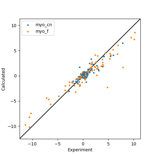
Finally a correlation plot is made.
#### Plot the correlation ####
from matplotlib import pyplot as plt
fig, ax = plt.subplots(figsize=(5,5))

# Plot the data correlations
ax.scatter(*zip(*compare_cn), s=7, label="myo_cn")
ax.scatter(*zip(*compare_f), s=7, label="myo_f")

# Plot a diagonal
l, h = ax.get_xlim()
ax.plot([l,h],[l,h],'-k',zorder=0)
ax.set_xlim(l,h)
ax.set_ylim(l,h)

# Make axis labels and save figure
ax.set_xlabel("Experiment")
ax.set_ylabel("Calculated")
ax.legend()
fig.savefig("ccr_calculate.png")
Output: [ccr_calculate.png]
