Fit spectral power density tensor
This example shows how to fit the spectral power density tensor to anisotropic PREs. The data and theory are derived from https://doi.org/10.1039/C8CP01332B.
Downloads
Download the data files
parashift_Tb.pdbandparashift_Tb_R1_exp.prefrom here:Download the script
pre_fit_aniso_dipolar.py
Script + Explanation
Load the relevant modules, read the PDB coordinates and experimental PRE values. Parse the values.
from paramagpy import protein, metal, fit, dataparse
from matplotlib import pyplot as plt
import numpy as np

prot = protein.load_pdb('../data_files/parashift_Tb.pdb')
pre_exp = dataparse.read_pre('../data_files/parashift_Tb_R1_exp.pre')
exp = prot.parse(pre_exp)
The spectral power density tensor is written here explicitly and set to the attribute g_tensor. The values here are sourced from the original paper, and arise from the robust linear fit to the experimental data. We will use this tensor for comparison to the fit achieved by paramagpy.
m = metal.Metal(taur=0.42E-9, B0=1.0, temperature=300.0)
m.set_lanthanide('Tb')

m.g_tensor = np.array([
	[1754.0, -859.0, -207.0],
	[-859.0, 2285.0, -351.0],
	[-207.0, -351.0, -196.0]]) * 1E-60
An starting tensor with no parameters is also initialised and will be used for fitting to the exerimental data with paramagpy.
m0 = metal.Metal(taur=0.42E-9, B0=1.0, temperature=300.0)
m0.set_lanthanide('Tb')
The fit is conducted by setting the usegsbm flag to True. This uses anisotropic SBM theory to fit the spectral power density tensor in place of the isotropic SBM theory. The relevant fitting parameters must be specified as 't1e', 'gax', 'grh', 'a','b','g' which represent the electronic relaxation time, the axial and rhombic componenets of the power spectral density tensor and the 3 Euler angles alpha, beta and gamma respectively. Note that the fitted t1e parameter is only an estimate of the electronic relaxation time.
[mfit], [data] = fit.nlr_fit_metal_from_pre([m0], [exp], params=('t1e', 'gax', 'grh', 'a','b','g'),
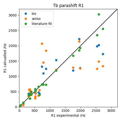
Finally the results of the fit are plotted alongside the isotropic theory and the literature fit. Note that the difference in the fit from paramagpy is small, and probably arises because the original paper uses a Robust linear fit, which may include weighting with experimental uncertainties. However paramagpy weights values evely here because the experimental uncertainties are unknown.
pos = np.array([a.position for a in exp['atm']])
gam = np.array([a.gamma for a in exp['atm']])

fig = plt.figure(figsize=(5,5))
ax = fig.add_subplot(111)
ax.plot([0,3200],[0,3200], '-k')
ax.plot(exp['exp'], mfit.fast_sbm_r1(pos, gam), marker='o', lw=0, label='iso')
ax.plot(exp['exp'], mfit.fast_g_sbm_r1(pos, gam), marker='o', lw=0, label='aniso')
ax.plot(exp['exp'], m.fast_g_sbm_r1(pos, gam), marker='o', lw=0, label='literature fit')
ax.set_xlim(0,3200)
ax.set_ylim(0,3200)
ax.set_xlabel("R1 experimental /Hz")
ax.set_ylabel("R1 calcualted /Hz")
ax.set_title("Tb parashift R1")
ax.legend()
fig.tight_layout()
fig.savefig("pre_fit_aniso_dipolar.png")
Output: [pre_fit_aniso_dipolar.png]