Constrained Fitting
This example shows how to fit a \({\Delta\chi}\)-tensor with constraints applied. The two cases here constrain position to fit a tensor to a known metal ion position form an X-ray structure, and fit an axially symmetric tensor with only 6 of the usual 8 parameters.
Downloads
Download the data files
4icbH_mut.pdbandcalbindin_Er_HN_PCS.npcfrom here:Download the script
pcs_fit_constrained.py
Script + Explanation
The necessary modules are imported and data is loaded
from paramagpy import protein, fit, dataparse, metal

# Load data
prot = protein.load_pdb('../data_files/4icbH_mut.pdb')
rawData = dataparse.read_pcs('../data_files/calbindin_Er_HN_PCS.npc')
parsedData = prot.parse(rawData)
mStart = metal.Metal()
The calcium ion from the X-ray structure is contained in a heteroatom of the PDB file. We set the starting position of the tensor to this position.
# Set the starting position to Calcium ion heteroatom in PDB
mStart.position = prot[0]['A'][('H_ CA', 77, ' ')]['CA'].position
To fit the the anisotropy and orientation without position, the linear PCS equation can be solved analytically by the SVD gridsearch method but using only one point with a radius of zero. The Q-factor is then calculated and the tensor is saved.
# Calculate tensor by SVD
[mFit], [data] = fit.svd_gridsearch_fit_metal_from_pcs(
	[mStart],[parsedData], radius=0, points=1)

qfac = fit.qfactor(data)

mFit.save('calbindin_Er_HN_PCS_tensor_position_constrained.txt')
Output: [pcs_fit_constrained.png]
ax    | 1E-32 m^3 :    -8.152
rh    | 1E-32 m^3 :    -4.911
x     |   1E-10 m :    25.786
y     |   1E-10 m :     9.515
z     |   1E-10 m :     6.558
a     |       deg :   125.841
b     |       deg :   142.287
g     |       deg :    41.758
mueff |        Bm :     0.000
shift |       ppm :     0.000
B0    |         T :    18.790
temp  |         K :   298.150
t1e   |        ps :     0.000
taur  |        ns :     0.000
To fit an axially symmetric tensor, we can used the Non-linear regression method and specify exactly which parameters we want to fit. This will be the axiality ax, two Euler angles b and g and the position coordinates. Note that in the output, the rhombic rh and alpha a parameters are redundant.
# Calculate axially symmetric tensor by NRL
[mFitAx], [dataAx] = fit.nlr_fit_metal_from_pcs(
	[mStart], [parsedData], params=('ax','b','g','x','y','z'))

qfacAx = fit.qfactor(dataAx)

mFitAx.save('calbindin_Er_HN_PCS_tensor_axially_symmetric.txt')
Output: [pcs_fit_constrained.png]
ax    | 1E-32 m^3 :     9.510
rh    | 1E-32 m^3 :     0.000
x     |   1E-10 m :    24.948
y     |   1E-10 m :     8.992
z     |   1E-10 m :     3.205
a     |       deg :     0.000
b     |       deg :   134.697
g     |       deg :   180.000
mueff |        Bm :     0.000
shift |       ppm :     0.000
B0    |         T :    18.790
temp  |         K :   298.150
t1e   |        ps :     0.000
taur  |        ns :     0.000
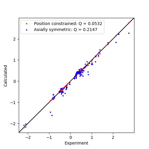
Finally we plot the data.
#### Plot the correlation ####
from matplotlib import pyplot as plt
fig, ax = plt.subplots(figsize=(5,5))

# Plot the data
ax.plot(data['exp'], data['cal'], marker='o', lw=0, ms=2, c='r',
	label="Position constrained: Q = {:5.4f}".format(qfac))

ax.plot(dataAx['exp'], dataAx['cal'], marker='o', lw=0, ms=2, c='b',
	label="Axially symmetric: Q = {:5.4f}".format(qfacAx))

# Plot a diagonal
l, h = ax.get_xlim()
ax.plot([l,h],[l,h],'-k',zorder=0)
ax.set_xlim(l,h)
ax.set_ylim(l,h)

# Make axis labels and save figure
ax.set_xlabel("Experiment")
ax.set_ylabel("Calculated")
ax.legend()
fig.savefig("pcs_fit_constrained.png")
Output: [pcs_fit_constrained.png]
