Fit Tensor to PDB with Models
This example shows how to fit a \({\Delta\chi}\)-tensor to experimental PCS data using an NMR structure that contains multiple models. Data for calbindin D9k are used as in the previous example Fit Tensor to PCS Data.
There are 3 fitting options available in paramagpy for fitting:
Averaged fit: A tensor is fit to each model independently, and then all fitted tensors are averaged together. This is a good choice if models in your PDB represent structural uncertainty.
Ensemble averaged fit: A single tensor is fit simultaneously to all models by averaging calculated PCS values during fitting. This is a good choice if models in your PDB represent dynamics as comes from a molecular dynamics simulation.
Separate model fit: A tensor is fit to each model independently and the best fitting model is taken. This is a good choice if you are only looking for the best fit model in a PDB containing many models.
Downloads
Download the data files
2bcb.pdbandcalbindin_Er_HN_PCS.npcfrom here:Download the script
pcs_fit_models.py
Script + Explanation
Firstly, the standard preamble and loading of data.
from paramagpy import protein, fit, dataparse, metal

# Load data
prot = protein.load_pdb('../data_files/2bcb.pdb')
rawData = dataparse.read_pcs('../data_files/calbindin_Er_HN_PCS.npc')
parsedData = prot.parse(rawData)
If all models are provided in the parsedData argument, the default functionality for all fitting methods such as paramagpy.fit.nlr_fit_metal_from_pcs() is to fit using method 1, meaning a tensor is fit to each model and the averaged tensor is returned. This is equivalent to setting the ensebleAverage argument to False. This is done below. Averaging behaviour can be controlled through the idx column of parsedData. The idx array contains common integers for corresponding atoms to be averaged, and defaults to the atom’s serial number found in the PDB file.
#### Averaged fit to all models ####
[mGuess], [data] = fit.svd_gridsearch_fit_metal_from_pcs([mStart], [parsedData], radius=10, points=10, ensembleAverage=False)
[mFit], [data] = fit.nlr_fit_metal_from_pcs([mGuess], [parsedData], ensembleAverage=False)
qfac = fit.qfactor(data, ensembleAverage=False)
avg = qfac, data, mFit
Method 2 can be followed by the same method, except setting the ensebleAverage argument to True. At each stage of the fitting process, all PCS calculations are then averaged before fitting of a single tensor to all the data simultaneously. The ensemble averaging behaviour can be set through the idx column of the input data for paramagpy.fit.nlr_fit_metal_from_pcs().
#### Ensembled averaged fit to all models ####
[mGuess], [data] = fit.svd_gridsearch_fit_metal_from_pcs([mStart], [parsedData], radius=10, points=10, ensembleAverage=True)
[mFit], [data] = fit.nlr_fit_metal_from_pcs([mGuess], [parsedData], ensembleAverage=True)
qfac = fit.qfactor(data, ensembleAverage=True)
e_avg = qfac, data, mFit
Method 3 can be achieved by constructing a for loop over the PDB models and fitting a separate tensor to the data from each model. The model which achieves the lowest Q-factor can then be extracted.
#### Seperate fit for each model ####
sep = {}
for model in prot:
    singleModelData = parsedData[parsedData['mdl']==model.id]
    [mGuess], [data] = fit.svd_gridsearch_fit_metal_from_pcs([mStart], [singleModelData], radius=10, points=10)
    [mFit], [data] = fit.nlr_fit_metal_from_pcs([mGuess], [singleModelData])
    qfac = fit.qfactor(data)
    sep[model.id] = qfac, data, mFit
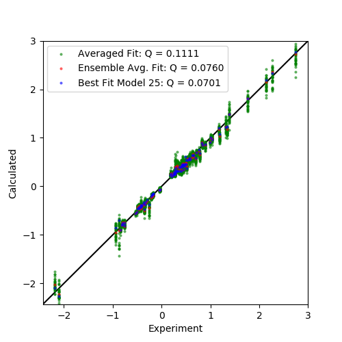
Finally we plot three sets of data:
The averaged fit calculated over all models (green)
The ensemble average of the calculated values of the ensemble fit (red)
The best fitting single model (blue)
Note that to calculate the ensemble average of the calculated values we use the function paramagpy.fit.ensemble_average(). This can take any number of arguments, and will average values based on common serial numbers of the list of atoms in the first argument.
#### Plot the correlation ####
from matplotlib import pyplot as plt
fig, ax = plt.subplots(figsize=(5,5))

# Plot averaged fit correlation
qfac, data, mFit = avg
mFit.save('calbindin_Er_HN_PCS_tensor_average.txt')
ax.plot(data['exp'], data['cal'], marker='o', lw=0, ms=2, c='g',
    alpha=0.5, label="Averaged Fit: Q = {:5.4f}".format(qfac))

# Plot ensemble averaged fit correlation
qfac, data, mFit = e_avg
mFit.save('calbindin_Er_HN_PCS_tensor_ensemble_average.txt')
# Ensemble average the data to get a single point for each model
data = fit.ensemble_average(data)
ax.plot(data['exp'], data['cal'], marker='o', lw=0, ms=2, c='r',
    alpha=0.5, label="Ensemble Avg. Fit: Q = {:5.4f}".format(qfac))

# Plot best fit model correlation
# Sort fits by Qfactor and take smallest
model, (qfac, data, mFit) = sorted(sep.items(), key=lambda x: x[1][0])[0]
mFit.save('calbindin_Er_HN_PCS_tensor_best_model.txt')
ax.plot(data['exp'], data['cal'], marker='o', lw=0, ms=2, c='b',
    alpha=0.5, label="Best Fit Model {}: Q = {:5.4f}".format(model, qfac))

# Plot a diagonal
l, h = ax.get_xlim()
ax.plot([l,h],[l,h],'-k',zorder=0)
ax.set_xlim(l,h)
ax.set_ylim(l,h)

# Make axis labels and save figure
ax.set_xlabel("Experiment")
ax.set_ylabel("Calculated")
ax.legend()
fig.savefig("pcs_fit_models.png")
Output: [pcs_fit_models.png]