Fit multiple PCS datasets to common position
This example shows how to fit multiple \({\Delta\chi}\)-tensors to their respective datasets with a common position, but varied magnitude and orientation. This may arise if several lanthanides were investigated at the same binding site, and the data may be used simultaneously to fit a common position. Data from several PCS datasets for calbindin D9k were used here, and is a generalisation of the previous example: Fit Tensor to PCS Data.
Downloads
Download the data files
4icbH_mut.pdb,calbindin_Tb_HN_PCS.npc,calbindin_Er_HN_PCS.npcandcalbindin_Yb_HN_PCS_tensor.txtfrom here:Download the script pcs_fit_multiple.py
Explanation
The protein and PCS datasets are loaded and parsed. These are placed into a list parsedData, for which each element is a PCS dataset of a given lanthanide.
The two fitting functions:
can accept a list of metal objects and a list of datasets with arbitrary size. If this list contains more than one element, fitting will be performed to a common position. The starting position is taken only from the first metal of the list.
After fitting, a list of fitted metals is returned. The fitted tensor are then written to files and a correlation plot is made.
Script
from paramagpy import protein, fit, dataparse, metal
# Load the PDB file
prot = protein.load_pdb('../data_files/4icbH_mut.pdb')
# Load the PCS data
rawData1 = dataparse.read_pcs('../data_files/calbindin_Tb_HN_PCS.npc')
rawData2 = dataparse.read_pcs('../data_files/calbindin_Er_HN_PCS.npc')
rawData3 = dataparse.read_pcs('../data_files/calbindin_Yb_HN_PCS.npc')
# Associate PCS data with atoms of the PDB
parsedData = []
for rd in [rawData1, rawData2, rawData3]:
parsedData.append(prot.parse(rd))
# Make a list of starting tensors
mStart = [metal.Metal(), metal.Metal(), metal.Metal()]
# Set the starting position to an atom close to the metal
mStart[0].position = prot[0]['A'][56]['CA'].position
# Calculate initial tensors from an SVD gridsearch
mGuess, datas = fit.svd_gridsearch_fit_metal_from_pcs(
mStart, parsedData, radius=10, points=10)
# Refine the tensors using non-linear regression
fitParameters = ['x','y','z','ax','rh','a','b','g']
mFit, datas = fit.nlr_fit_metal_from_pcs(mGuess, parsedData, fitParameters)
# Save the fitted tensors to files
for name, metal in zip(['Tb','Er','Yb'], mFit):
metal.save("tensor_{}.txt".format(name))
#### Plot the correlation ####
from matplotlib import pyplot as plt
fig, ax = plt.subplots(figsize=(5,5))
# Plot the data
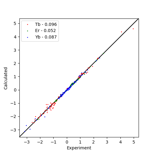
for d, name, colour in zip(datas, ['Tb','Er','Yb'],['r','g','b']):
qfactor = fit.qfactor(d)
ax.plot(d['exp'], d['cal'], marker='o', lw=0, ms=1, c=colour,
label="{0:} - {1:5.3f}".format(name, qfactor))
# Plot a diagonal
l, h = ax.get_xlim()
ax.plot([l,h],[l,h],'-k',zorder=0)
ax.set_xlim(l,h)
ax.set_ylim(l,h)
# Axis labels
ax.set_xlabel("Experiment")
ax.set_ylabel("Calculated")
ax.legend()
fig.savefig("pcs_fit_multiple.png")
Outputs
Tb fitted tensor
ax    | 1E-32 m^3 :    31.096
rh    | 1E-32 m^3 :    12.328
x     |   1E-10 m :    25.937
y     |   1E-10 m :     9.481
z     |   1E-10 m :     6.597
a     |       deg :   151.053
b     |       deg :   152.849
g     |       deg :    69.821
mueff |        Bm :     0.000
shift |       ppm :     0.000
B0    |         T :    18.790
temp  |         K :   298.150
t1e   |        ps :     0.000
taur  |        ns :     0.000
Er fitted tensor
ax    | 1E-32 m^3 :    -8.422
rh    | 1E-32 m^3 :    -4.886
x     |   1E-10 m :    25.937
y     |   1E-10 m :     9.481
z     |   1E-10 m :     6.597
a     |       deg :   126.015
b     |       deg :   142.899
g     |       deg :    41.039
mueff |        Bm :     0.000
shift |       ppm :     0.000
B0    |         T :    18.790
temp  |         K :   298.150
t1e   |        ps :     0.000
taur  |        ns :     0.000
Yb fitted tensor
ax    | 1E-32 m^3 :    -5.392
rh    | 1E-32 m^3 :    -2.490
x     |   1E-10 m :    25.937
y     |   1E-10 m :     9.481
z     |   1E-10 m :     6.597
a     |       deg :   129.650
b     |       deg :   137.708
g     |       deg :    88.796
mueff |        Bm :     0.000
shift |       ppm :     0.000
B0    |         T :    18.790
temp  |         K :   298.150
t1e   |        ps :     0.000
taur  |        ns :     0.000
Correlation Plot
